Covolution Neural Network

 CONVOLUTIONAL NEURAL NETWORK(CNN)

 

The CNN is an algorithm mainly designed to work on the images, where an image is internally nothing but the set of pixel values, that is for example if you say you have a color image of 48x48 size which internally means you have 6912(48x48x3=6912) pixel values, where 3 indicates the RGB channels, Similarly, if you consider the black and white image of size 48x48, then it means you have 2304(48x48x1=2304) pixel values in your image, where 1 indicates gray channel.

                     

                                     Image reference: https://en.wikipedia.org/wiki/Grayscale

 

WORKING OF CNN:

The CNN algorithm works in form of layers. Where the most important layer is called the convolution layer. In this layer, we use a concept called filters. The working of this layer is very simple that is, when you consider an image in the training stage the algorithm tries to learn some filters on the image, where filters are nothing but some feature values that correspond to the prediction of the output. To understand that let’s see an image example

                   Image reference:https://www.tensorflow.org/images/MNIST-Matrix.png

 

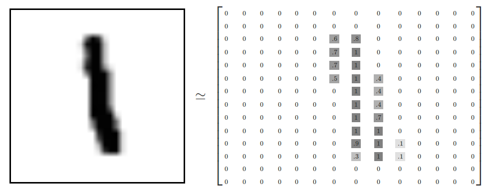
 Here when you try to see the image on the left side that is a handwritten character 1, whereas when you see the right side you can see the grayscale pixel values for the image. Where we can see that except for the place where the value 1 is present, remaining all are zeros.

In this, we can represent any image in the form of pixel values. Note, here the image is grayscale so it has pixel values in 1-D. If it is a color image, then it is going to have in a 3-D array (where one array for R, one for G, one for B).

Similarly, a filter is also nothing but a collection of values in a matrix

   

Image reference: https://medium.com/@RaghavPrabhu/understanding-of-convolutional-neural-network-cnn-deep-learning-99760835f148

 

As we can see in the images these filters can be different for different categories based on our

input and output. They are data specific and are trained by the algorithm.

As I said previously these filters are learned from the training data based on our output

requirement. The process of identifying filters is done internally by the model itself, we just

have to mention the number of filters and size of filters that we want.

 Coming to how the filters are useful, they are used to identify a certain feature in the test data or the test image. The entire process will be like this

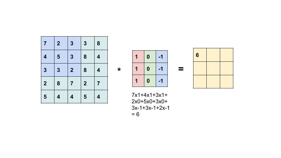
CONVOLUTION LAYER:

Now let’s see how filters internally work. Let's try to see in the steps

• First, the filter is placed on the image
• Now we multiply each value in the filter with each corresponding value of the image.
• Now we add up all the values that we got in the previous step and fill them in the corresponding
• position in the resultant matrix.

·        Similarly, we will move the filter based on the stride given or the required stride 

Image reference: https://learnopencv.com/wp-content/uploads/2017/11/convolution-example-matrix.gif

Here when you try to see the dark blue shade on the first array indicates filters.

Stride:

Stride is nothing but the movement of filters, here when you try to see the filter is moving one position left and then later one position down. Because by default stride is set to 1. If you want to have two positions left and two positions down then we will change stride to 2.

Imagereference:https://1.bp.blogspot.com/xzQJ7bxlCUk/XkrIwVmHRI/AAAAAAAAAqg/CKNuwo6V01EeTMDrNwD9g-3sqYbwur0gwCLcBGAsYHQ/s1600/appendix_C_eg_1.png

Then there is another term that we need to discuss which is padding. In the above images when we are applying convolution or filters, we can see that we are losing some information in the output that is when we are taking a 6x6 image and applying a 2x2 kernel, the output is a 3x3 matrix or image. This means we are losing some information. Then there arrives a question “how to prevent this data loss?”

 

There is one more key point here that we need to consider regarding padding, that is when we are applying a filter over the image, we can see that the edge values are getting covered under the filter only once, whereas the remaining values are getting covered more than once. This may cause a loss of information that is present on the edges. We can see this in the above images where we discussed stride. This issue can also be solved by padding.

Padding: 

Padding is nothing but adding some extra layers over the image to prevent the image from data loss. We will add padding over the data based on our requirement, that is if padding is kept as 1 which means we are going to add a row of 0's or -1's at the top, bottom, left, and right of the image matrix. 

                                    Image reference: http://xrds.acm.org/blog/wp-content/uploads/2016/06/Figure_3.png

POOLING LAYER:

Now we have to see one more layer which is the max-pooling layer. The main use of the max-pooling layer is to reduce the image size. This is used to reduce the heavy computation for the processor.

There are two types of max pooling techniques:

•        Max pooling
•       Average pooling

Max pooling:

It is a technique where a filter is applied to the image and the maximum value within the filter is taken as a new value in the corresponding output cell.

Average pooling:

 It is a technique where a filter is applied to the image and the average value of all the elements within the filter is taken as a new value in the corresponding output cell.

 Image reference: 

https://www.researchgate.net/publication/333593451/figure/fig2/AS:765890261966848@1559613876098/Illustration-of-Max-Pooling-and-Average-Pooling-Figure-2-above-shows-an-example-of-max.png

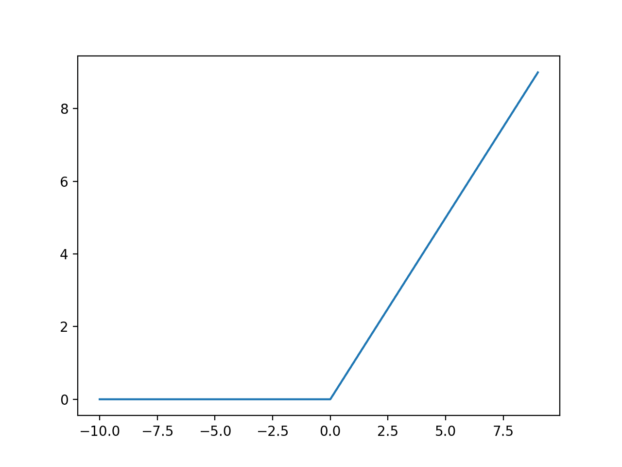
Now we need to learn about one small thing called the activation function. 

The activation functions are those which are used to simplify the output that comes after applying the convolution layer. There are many activation functions among them the most famous function that we are going to use in the paper is relu.

RELU:

The working of the relu function is so simple. The function result is 0 for all the negative values and the absolute value for all the positive values.

Image reference: https://machinelearningmastery.com/wp-content/uploads/2018/10/Line-Plot-of-Rectified-Linear-Activation-for-Negative-and-Positive-Inputs.png

Image reference: https://pylessons.com/media/Tutorials/Tensorflow-Keras-tutorials/CNN-tutorial-introduction/Figure_11.jpg

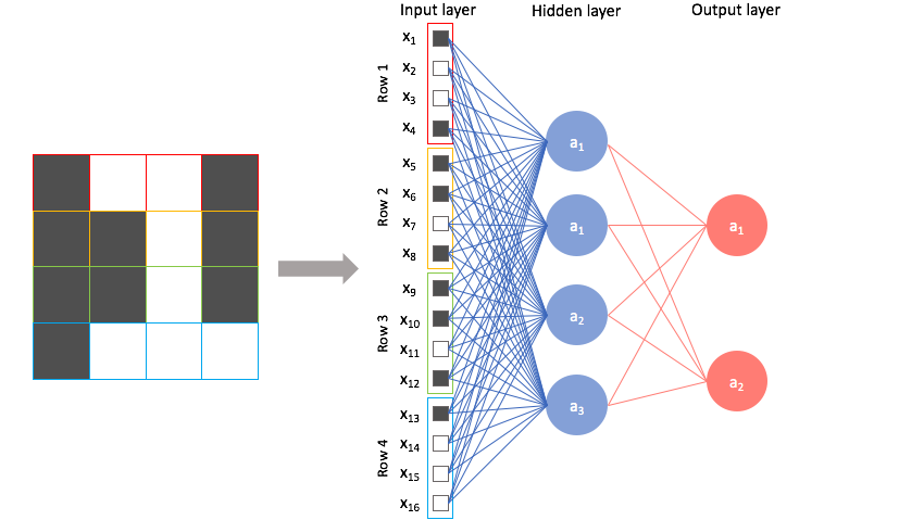
FLATTEN LAYER:

Here all the data from the different feature maps are converted into a single one- dimensional array and then passed to a fully connected network or dense network.

Image reference: https://sds-platform-private.s3-us-east-2.amazonaws.com/uploads/73_blog_image_1.png

FULLY CONNECTED OR DENSE LAYER:

 In this, we will use a fully connected neural network with each layer consisting of the required number of neurons. And we will pass the flattened array as input to the first neuron layer. And we will have n number of neuron layers based on the requirement. Where each layer consists of user-specified neurons. The neurons in the output layer must be equal to the number of output classes that you want. Where each neuron in the output layer corresponds to each class. This is called a fully connected layer because all neurons of one layer are connected to all neurons of the next layer. The main task here is to find the weights on the neuron links.

Image reference: https://www.jeremyjordan.me/content/images/2017/07/Screen-Shot-2017-07-27-at-12.07.11-AM.png

IMPLEMENTATION PART:

Dataset:

The dataset is collected from the Kaggle website. This dataset consists of lung X-ray images of patients. The dataset consists of 5216 training images, out of which 1341 are no Pneumonia affected people X-ray scans, and 3875 are scans of people having Pneumonia. And the test dataset consists of 234 normal people scans and 390 scans of Pneumonia affected people. The size of each image is considered 224X224X3. The dataset credit goes to

https://www.kaggle.com/datasets/paultimothymooney/chest-xray-pneumonia

Normal X-ray

 

Pneumonia-affected person X-ray

RESULTS:

While coming to the application part we are considering a total of 5216 lung X-ray scans and out of 1341 are normal people scans and 3875 are scans of the Pneumonia affected people. The data may be slightly unbalanced, but it's just fine for image data like this. Here we are much concentrated on disease prediction.

The image size that we are considering is 224x224 and with an RGB channel.

The CNN architecture that we initially used is 

With the above architecture when the model is tried it yielded approximately 74% after 10 epochs (10 rounds in simple terms).

Now we will try to change the architecture and try to see the same thing with a different view. This architecture that we have used is similar to VGG-16 architecture(A pre-trained model by google).

Here we have a good point to learn that even the change of architecture, sometimes can't yield good accuracy. In the above image, you can see that even when we used the similar architecture of VGG-16 it doesn't yield good accuracy. And we can see that there is a drop in accuracy by almost 50%. From this the main finding is there is no hard and fast rule for producing accuracy, it is just a trial and error process.

CONCLUSION:

While coming to traditional CNN the architecture is flexible, that is there is no fixed rule for the number or type, or order of layers and even there is no hard and fast rule for the number of kernels, size of kernels, or several neurons in dense layer. The only way to pick a model is by applying all layers by trial and error method and picking a model that betters generates high accuracy and satisfies the requirements.